Starting the environment
Once QMflows has been installed the user should run the following command to initialize the environment:
[user@int1 ~]$ source activate qmflows
discarding /home/user/anaconda3/bin from PATH
prepending /home/user/anaconda3/envs/qmflows/bin to PATH
(qmflows)[user@int1 ~]$ python --version
Python 3.5.2 :: Anaconda custom (64-bit)
To leave the environment the following command is used
(qmflows)[user@int1 ~]$ source deactivate
discarding /home/user/anaconda3/envs/qmflows/bin from PATH
To finalize preparations before running QMflows: if you don’t want the results to end up in the current work directory, create a new results folder.
[26]:
mkdir tutorial_results
What is QMflows?
QMflows is a python library that enables executing complicated workflows of interdependent quantum chemical (QM) calculations in python. It aims at providing a common interface to multiple QM packages, enabling easy and systematic generation of the calculation inputs, as well as facilitating automatic analysis of the results. Furthermore it is build on top of the powerful Noodles framework for executing the calculations in parallel where possible.
The basics: calling packages
Currently QMFLOWS offers an interface with the following simulation software:
SCM (ADF and DTFB)
CP2K
ORCA
Note:
Please make sure that the packages you want to use in QMflows are installed and active; in most supercomputer the simulation package are available using a command like (consult your system administrator):
load module superAwesomeQuantumPackage/3.1421Also some simulation packages required that you configure a scratch folder. For instance Orca requires a SCR folder to be defnied while ADF called it SCM_TMPDIR.
With qmflows you can write a python script that simply calls one of the package objects adf, dftb, cp2k, or orca. As arguments to the call, you need to provide a settings objects defining the input of a calculation, a molecular geometry, and, optionally, a job name that enables you to find back the “raw” data of the calculation later on.
Let’s see how this works:
First we define a molecule, for example by reading one from an xyz file:
[7]:
from scm.plams import Molecule
acetonitrile = Molecule("../test/test_files/molecules/acetonitrile.xyz")
print(acetonitrile)
  Atoms:
    1         C      2.366998      0.579794     -0.000000
    2         C      1.660642      1.834189      0.000000
    3         N      1.089031      2.847969      0.000000
    4         H      2.100157      0.010030      0.887206
    5         H      2.100157      0.010030     -0.887206
    6         H      3.439065      0.764079     -0.000000
Then we can perform geometry optimization on the molecule by a call to the dftb package object:
[8]:
from qmflows import dftb, templates, run
job = dftb(templates.geometry, acetonitrile, job_name="dftb_geometry_optimization")
print(job)
<noodles.interface.decorator.PromisedObject object at 0x7ff8fe871da0>
As you can see, “job” is a so-called “promised object”. It means it first needs to be “run” by the Noodles scheduler to return a normal python object.
[29]:
result = run(job, path="tutorial_results", folder="run_one", cache="tutorial_cache.json")
print(result)
[09:14:04] PLAMS working folder: /home/lars/workspace/qmflows/jupyterNotebooks/tutorial_results/run_one
╭─(running jobs)
│ Running dftb dftb_geometry_optimization...
╰(✔)─(success)
<qmflows.packages.SCM.DFTB_Result object at 0x7f6c8e30bcf8>
We can easily retrieve the calculated properties from the DFTB calculation such as the dipole or the optimized geometry for use in subsequent calculations.
[30]:
print("Dipole: ", result.dipole)
print(result.molecule)
Dipole:  [1.0864213029, -1.9278296041, -0.0]
  Atoms:
    1         C      2.366998      0.579794     -0.000000
    2         C      1.660642      1.834189      0.000000
    3         N      1.089031      2.847969      0.000000
    4         H      2.100157      0.010030      0.887206
    5         H      2.100157      0.010030     -0.887206
    6         H      3.439065      0.764079     -0.000000
Settings and templates
In the above example templates.geometry was actually a predefined Settings object. You can define and manipulate Settings in a completely flexible manner as will be explained in this section. To facilitate combining different packages in one script, QMflows defines a set of commonly used generic keywords, which can be combined with package specific keywords, to provide maximum flexibility.
[10]:
from qmflows import Settings
s = Settings()
s.basis = "DZP"
s.specific.adf.basis.core = "large"
s.freeze = [1,2,3]
print(s)
basis:  DZP
specific:
         adf:
             basis:
                   core:        large
freeze:         [1, 2, 3]
This code snippet illustrates that the Settings can be specified in two ways, using generic or specific keywords. Generic keywords represent input properties that are present in most simulation packages like a basis set while specific keywords allow the user to apply specific keywords for a package that are not in a generic dictionary.
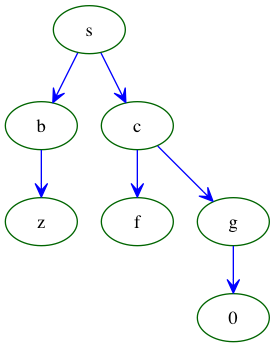
Expert info:
Settings are a subclass of python dictionaries to represent herarchical structures, like
[3]:
from IPython.display import Image
Image(filename="files/simpleTree.png")
[3]:
In QMflows/PLAMS multiple settings objects can be combined using the
overlayfunction.
[11]:
merged_settings = templates.geometry.overlay(s)
print(merged_settings)
specific:
         adf:
             basis:
                   type:        SZ
                   core:        large
             geometry:
                      optim:    delocal
             numericalquality:  good
             scf:
                 converge:      1e-6
                 iterations:    100
         ams:
             ams:
                 GeometryOptimization:
                                      MaxIterations:    500
                 Task:  GeometryOptimization
         cp2k:
              force_eval:
                         dft:
                             mgrid:
                                   cutoff:      400
                                   ngrids:      4
                             qs:
                                method:         gpw
                             scf:
                                 OT:
                                    N_DIIS:     7
                                    minimizer:  DIIS
                                    preconditioner:     full_single_inverse
                                 eps_scf:       1e-06
                                 max_scf:       200
                                 scf_guess:     atomic
                         subsys:
                                cell:
                                     periodic:  xyz
              global:
                     print_level:       low
                     project:   cp2k
                     run_type:  geometry_optimization
              motion:
                     geo_opt:
                             max_iter:  500
                             optimizer:         bfgs
                             type:      minimization
         cp2k_mm:
                 force_eval:
                            method:     FIST
                            mm:
                               forcefield:
                                          do_nonbonded:
                                          ei_scale14:   1.0
                                          ignore_missing_critical_params:
                                          shift_cutoff:         .TRUE.
                                          spline:
                                                 r0_nb:         0.25
                                          vdw_scale14:  1.0
                               poisson:
                                       ewald:
                                             ewald_type:        NONE
                                       periodic:        NONE
                               print:
                                     ff_info low:
                                                 spline_data:   .FALSE.
                                                 spline_info:   .FALSE.
                            subsys:
                                   cell:
                                        abc:    [angstrom] 50.0 50.0 50.0
                                        periodic:       NONE
                                   topology:
                                            center_coordinates:
                                                               center_point:    0.0 0.0 0.0
                                            coord_file_format:  OFF
                 global:
                        print_level:    low
                        project:        cp2k
                        run_type:       geometry_optimization
                 motion:
                        geo_opt:
                                max_iter:       500
                                optimizer:      lbfgs
                                type:   minimization
         dftb:
              dftb:
                   resourcesdir:        DFTB.org/3ob-3-1
              task:
                   runtype:     GO
         orca:
              basis:
                    basis:      sto_sz
              method:
                     functional:        lda
                     method:    dft
                     runtyp:    opt
basis:  DZP
freeze:         [1, 2, 3]
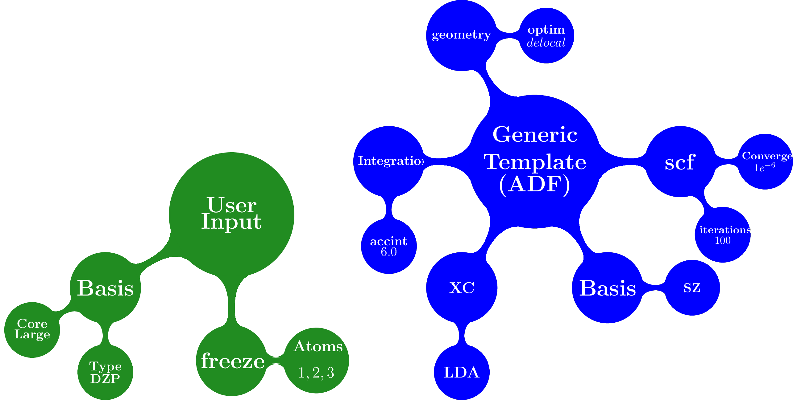
The overlay method merged the template containing default settings for geometry optimizations with different packages with the arguments provided by the user
[2]:
Image(filename="files/merged.png")
[2]:
resulting in:
[3]:
Image(filename="files/result_merged.png")
[3]:
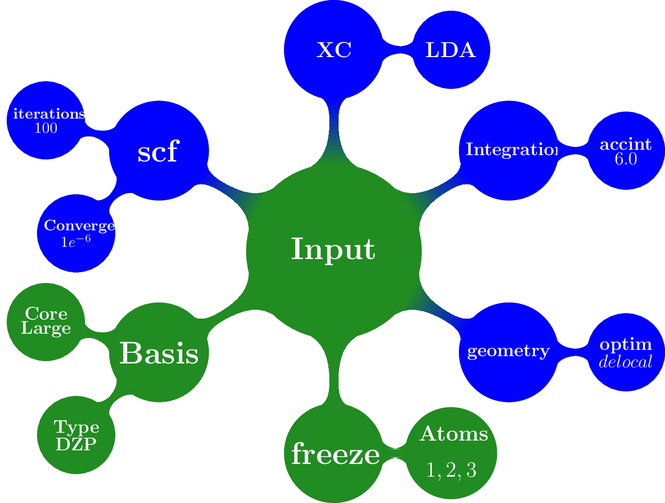
Note that the generic and specific keywords still exist next to each other and may not be consistent (e.g. different basis sets are defined in generic and specific keywords). Upon calling a package with a Settings object, the generic keywords are first translated into package specific keywords and combined with the relevant user defined specific keywords. In this step, the settings defined in generic keywords take preference. Subsequently, the input file(s) for the given package is/are generated, based on the keywords after specific.[package] based on the PLAMS software.
[12]:
from qmflows import adf
print(adf.generic2specific(merged_settings))
basis:  DZP
freeze:         [1, 2, 3]
specific:
         adf:
             basis:
                   core:        large
                   type:        DZP
             geometry:
                      optim:    cartesian
             numericalquality:  good
             scf:
                 converge:      1e-6
                 iterations:    100
             constraints:
                         atom 1:
                         atom 2:
                         atom 3:
         ams:
             ams:
                 GeometryOptimization:
                                      MaxIterations:    500
                 Task:  GeometryOptimization
         cp2k:
              force_eval:
                         dft:
                             mgrid:
                                   cutoff:      400
                                   ngrids:      4
                             qs:
                                method:         gpw
                             scf:
                                 OT:
                                    N_DIIS:     7
                                    minimizer:  DIIS
                                    preconditioner:     full_single_inverse
                                 eps_scf:       1e-06
                                 max_scf:       200
                                 scf_guess:     atomic
                         subsys:
                                cell:
                                     periodic:  xyz
              global:
                     print_level:       low
                     project:   cp2k
                     run_type:  geometry_optimization
              motion:
                     geo_opt:
                             max_iter:  500
                             optimizer:         bfgs
                             type:      minimization
         cp2k_mm:
                 force_eval:
                            method:     FIST
                            mm:
                               forcefield:
                                          do_nonbonded:
                                          ei_scale14:   1.0
                                          ignore_missing_critical_params:
                                          shift_cutoff:         .TRUE.
                                          spline:
                                                 r0_nb:         0.25
                                          vdw_scale14:  1.0
                               poisson:
                                       ewald:
                                             ewald_type:        NONE
                                       periodic:        NONE
                               print:
                                     ff_info low:
                                                 spline_data:   .FALSE.
                                                 spline_info:   .FALSE.
                            subsys:
                                   cell:
                                        abc:    [angstrom] 50.0 50.0 50.0
                                        periodic:       NONE
                                   topology:
                                            center_coordinates:
                                                               center_point:    0.0 0.0 0.0
                                            coord_file_format:  OFF
                 global:
                        print_level:    low
                        project:        cp2k
                        run_type:       geometry_optimization
                 motion:
                        geo_opt:
                                max_iter:       500
                                optimizer:      lbfgs
                                type:   minimization
         dftb:
              dftb:
                   resourcesdir:        DFTB.org/3ob-3-1
              task:
                   runtype:     GO
         orca:
              basis:
                    basis:      sto_sz
              method:
                     functional:        lda
                     method:    dft
                     runtyp:    opt
In the case of adf the above keywords result in the following input file for ADF package:
[34]:
adf_job = adf(merged_settings, acetonitrile, job_name='adf_acetonitrile')
result = run(adf_job, path="tutorial_results",
             folder="run_two", cache="tutorial_cache.json")
print(open('tutorial_results/run_two/adf_acetonitrile/adf_acetonitrile.in').read())
[09:14:04] PLAMS working folder: /home/lars/workspace/qmflows/jupyterNotebooks/tutorial_results/run_two
╭─(running jobs)
│ Running adf adf_acetonitrile...
(✔)╰─(success)
atoms
      1         C      2.419290      0.606560      0.000000
      2         C      1.671470      1.829570      0.000000
      3         N      1.065290      2.809960      0.000000
      4         H      2.000000      0.000000      1.000000
      5         H      2.000000      0.000000     -1.000000
      6         H      3.600000      0.800000      0.000000
end

basis
  core large
  type DZP
end

constraints
  atom 2
  atom 3
  atom 4
end

geometry
  optim cartesian
end

integration
  accint 6.0
end

scf
  converge 1e-06
  iterations 100
end

xc
  lda
end

end input
Combining multiple jobs
Multiple jobs can be combined, while calling the run function only once. The script below combines components outlined above:
[35]:
from scm.plams import Molecule
from qmflows import dftb, adf, templates, run, Settings

acetonitrile = Molecule("files/acetonitrile.xyz")

dftb_opt = dftb(templates.geometry, acetonitrile, job_name="dftb_opt")

s = Settings()
s.basis = "DZP"
s.specific.adf.basis.core = "large"
adf_single = adf(templates.singlepoint.overlay(s), dftb_opt.molecule, job_name="adf_single")

adf_result = run(adf_single, path="tutorial_results", folder="workflow", cache="tutorial_cache.json")
print(adf_result.molecule)
print(adf_result.energy)
[09:15:08] PLAMS working folder: /home/lars/workspace/qmflows/jupyterNotebooks/tutorial_results/workflow
╭─(running jobs)
│ Running dftb dftb_opt...
(✔)│ Running adf adf_single...
(✔)╰─(success)
  Atoms:
    1         C      0.000000      0.000000      0.656511
    2         C      0.000000      0.000000     -0.783088
    3         N      0.000000      0.000000     -1.946913
    4         H     -0.512221     -0.887193      1.022016
    5         H      1.024442      0.000000      1.022016
    6         H     -0.512221      0.887193      1.022016

-1.4094874734528888
In this case the second task adf_single reads the molecule optimized in the first job dftb_opt. Note that dftb_opt as well as dftb_opt.molecule are promised objects. When run is applied to the adf_single job, noodles builds a graph of dependencies and makes sure all the calculations required to obtain adf_result are performed.
All data related to the calculations, i.e. input files generated by QMflows and the resulting output files generated by the QM packages are stored in folders named after the job_names, residing inside a results folder:
[36]:
ls tutorial_results
run_one/ run_two/ workflow/
[37]:
ls tutorial_results/workflow
adf_single/ dftb_opt/ workflow.log
[38]:
ls tutorial_results/workflow/adf_single
adf_single.dill  adf_single.in   adf_single.run*  logfile  t21.H
adf_single.err   adf_single.out  adf_single.t21   t21.C    t21.N
[ ]: