Further Reading
Generic Keywords
Quantum chemistry packages use gaussian type orbitals (GTO) or slater type orbitals (STO) to perform the simulation. The packages use the same standards for the basis set and it will be really handy if we can defined a “generic” keyword for basis sets. Fortunately qmflows already offers such keyword that can be used among the packages that use the same basis standard,
[11]:
from qmflows import Settings
s = Settings()
s.basis = "DZP"
Internally QMflows will create a hierarchical structure representing basis DZP for the packages that can handle that basis set. Other generic keyowrds like: functional, inithess, etc. have been implemented.
The Following table describes some of the available generic keywords and the Packages where the funcionality is implemented
Generic Keyword |
Packages |
Description |
|---|---|---|
basis |
ADF, CP2K, Orca |
Set the basis set |
potential |
CP2K |
Set the pseudo potential |
cell_angles |
CP2K |
Specified the angles of the unit cell |
cell_parameters |
CP2K |
Specified the vectors of the unit cell |
constraint |
ADF, Orca |
Constrain the distance, angle or dihedral angle for a set of molecules |
freeze |
ADF, Orca |
Freeze a set of atoms indicated by their indexes or symbols |
functional |
ADF, CP2K |
Set the DFT functional |
inithess |
ADF, Orca |
Provide an initial Hessian matrix |
optimize |
ADF, DFTB, Orca |
Perform a molecular optimization |
selected_atoms |
ADF, Orca |
Optimize the given set of atoms while keeping the rest fixed |
ts |
ADF, DFTB, Orca |
Carry out a transition state optimization |
Note: QMflows Does not have chemical intuition and if you provide a meaningless keyword, like a wrong basis set it will not warm you.
Templates
As has been shown so far, Settings can be specified in two ways: generic or specific. Generic keywords represent input properties that are present in most simulation packages like a basis set while specific keywords resemble the input structure of a given package.
Generic and Specific Settings can express both simple and complex simulation inputs, but it would be nice if we can pre-defined a set of templates for the most common quantum chemistry simulations like: single point calculations, geometry optimizations, transition state optimization, frequency calculations, etc. qmflows already has a pre-defined set of templates containing some defaults that the user can modify for her/his own purpose. Templates are stored inside the
qmflows.templates module and are load from JSON files. A JSON file is basically a nested dictionary that is translated to a Settings object by qmflows.
Below it is shown the defaults for single point calculation
[1]:
from qmflows import templates
templates.singlepoint
RDKit WARNING: [16:43:01] Enabling RDKit 2019.09.1 jupyter extensions
[1]:
specific:
         adf:
             basis:
                   type:        SZ
             numericalquality:  normal
             scf:
                 converge:      1e-6
                 iterations:    100
         ams:
             ams:
                 Task:  SinglePoint
         dftb:
              dftb:
                   resourcesdir:        DFTB.org/3ob-3-1
              task:
                   runtype:     SP
         cp2k:
              force_eval:
                         dft:
                             mgrid:
                                   cutoff:      400
                                   ngrids:      4
                             print:
                                   mo:
                                      add_last:         numeric
                                      each:
                                           qs_scf:      0
                                      eigenvalues:
                                      eigenvectors:
                                      filename:         ./mo.data
                                      ndigits:  36
                                      occupation_numbers:
                             qs:
                                method:         gpw
                             scf:
                                 eps_scf:       1e-06
                                 max_scf:       200
                                 scf_guess:     restart
                         subsys:
                                cell:
                                     periodic:  xyz
              global:
                     print_level:       low
                     project:   cp2k
                     run_type:  energy
         cp2k_mm:
                 force_eval:
                            method:     FIST
                            mm:
                               print:
                                     ff_info low:
                                                 spline_data:   .FALSE.
                                                 spline_info:   .FALSE.
                               forcefield:
                                          ei_scale14:   1.0
                                          vdw_scale14:  1.0
                                          ignore_missing_critical_params:
                                          do_nonbonded:
                                          shift_cutoff:         .TRUE.
                                          spline:
                                                 r0_nb:         0.25
                               poisson:
                                       periodic:        NONE
                                       ewald:
                                             ewald_type:        NONE
                            subsys:
                                   cell:
                                        abc:    [angstrom] 50.0 50.0 50.0
                                        periodic:       NONE
                                   topology:
                                            coord_file_format:  OFF
                                            center_coordinates:
                                                               center_point:    0.0 0.0 0.0
                 global:
                        print_level:    low
                        project:        cp2k
                        run_type:       energy
         orca:
              method:
                     method:    dft
                     functional:        lda
              basis:
                    basis:      sto_sz
_ipython_canary_method_should_not_exist_:
The question is then, how I can modify a template with my own changes?
Suppose you are perfoming a bunch of constrained DFT optimizations using ADF . You need first to define a basis set and the constrains.
[3]:
from qmflows import Settings
s = Settings()
# Basis
s.basis = "DZP"
s.specific.adf.basis.core = "Large"

# Constrain
s.freeze = [1, 2, 3]
We use two generic keywords: freeze to indicate a constrain and basis to provide the basis set. Also, we introduce an specific ADF keywords core = Large. Now you merge your Settings with the correspoding template to carry out molecular geometry optimizations, using a method called overlay.
[4]:
from qmflows import templates
inp = templates.geometry.overlay(s)
The overlay method takes as input a template containing a default set for different packages and also takes the arguments provided by the user, as shown schematically 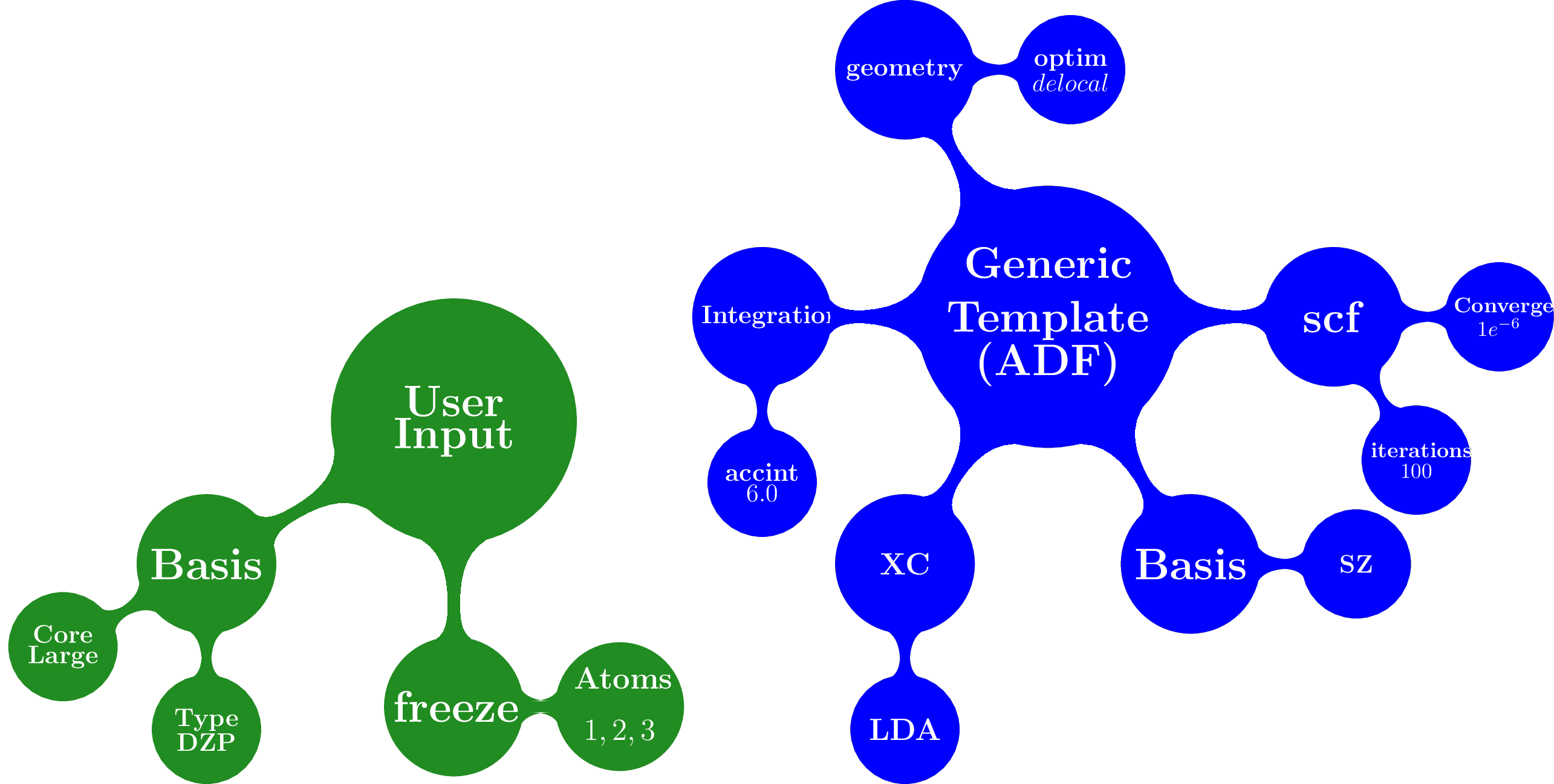
This overlay method merged the defaults for a given packages (ADF in this case) with the input supplied by the user, always given preference to the user input 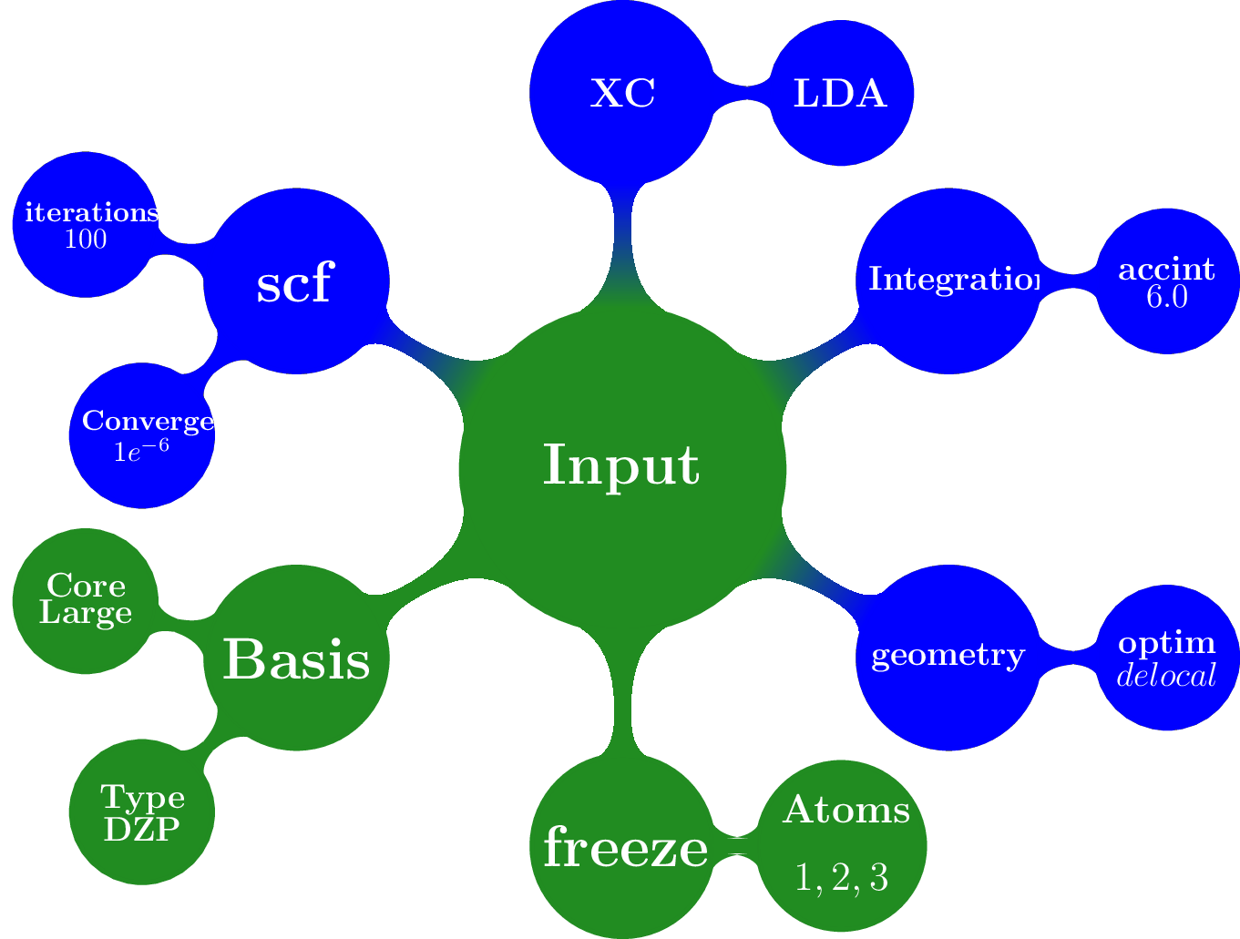
Below it is shown a combination of templates, generic and specific keywords to generate the input for a CP2K job
[2]:
from qmflows import templates

# Template
s = templates.singlepoint

# Generic keywords
s.cell_angles = [90.0, 90.0, 90.0]
s.cell_parameters=  38.0
s.basis = 'DZVP-MOLOPT-SR-GTH'
s.potential ='GTH-PBE'

# Specific Keywords
s.specific.cp2k.force_eval.dft.scf.max_scf  = 100
s.specific.cp2k.force_eval.subsys.cell.periodic = 'None'

print(s)
specific:
         adf:
             basis:
                   type:        SZ
             numericalquality:  normal
             scf:
                 converge:      1e-6
                 iterations:    100
         ams:
             ams:
                 Task:  SinglePoint
         dftb:
              dftb:
                   resourcesdir:        DFTB.org/3ob-3-1
              task:
                   runtype:     SP
         cp2k:
              force_eval:
                         dft:
                             mgrid:
                                   cutoff:      400
                                   ngrids:      4
                             print:
                                   mo:
                                      add_last:         numeric
                                      each:
                                           qs_scf:      0
                                      eigenvalues:
                                      eigenvectors:
                                      filename:         ./mo.data
                                      ndigits:  36
                                      occupation_numbers:
                             qs:
                                method:         gpw
                             scf:
                                 eps_scf:       1e-06
                                 max_scf:       100
                                 scf_guess:     restart
                         subsys:
                                cell:
                                     periodic:  None
              global:
                     print_level:       low
                     project:   cp2k
                     run_type:  energy
         cp2k_mm:
                 force_eval:
                            method:     FIST
                            mm:
                               print:
                                     ff_info low:
                                                 spline_data:   .FALSE.
                                                 spline_info:   .FALSE.
                               forcefield:
                                          ei_scale14:   1.0
                                          vdw_scale14:  1.0
                                          ignore_missing_critical_params:
                                          do_nonbonded:
                                          shift_cutoff:         .TRUE.
                                          spline:
                                                 r0_nb:         0.25
                               poisson:
                                       periodic:        NONE
                                       ewald:
                                             ewald_type:        NONE
                            subsys:
                                   cell:
                                        abc:    [angstrom] 50.0 50.0 50.0
                                        periodic:       NONE
                                   topology:
                                            coord_file_format:  OFF
                                            center_coordinates:
                                                               center_point:    0.0 0.0 0.0
                 global:
                        print_level:    low
                        project:        cp2k
                        run_type:       energy
         orca:
              method:
                     method:    dft
                     functional:        lda
              basis:
                    basis:      sto_sz
_ipython_canary_method_should_not_exist_:
cell_angles:    [90.0, 90.0, 90.0]
cell_parameters:        38.0
basis:  DZVP-MOLOPT-SR-GTH
potential:      GTH-PBE
Molecule
The next component to carry out a simulation is a molecular geometry. qmflows offers a convinient way to read Molecular geometries using the Plams library in several formats like: xyz , pdb, mol, etc.
[6]:
from scm.plams import Molecule
acetonitrile = Molecule("../test/test_files/acetonitrile.xyz")
print(acetonitrile)
  Atoms:
    1         C      2.366998      0.579794     -0.000000
    2         C      1.660642      1.834189      0.000000
    3         N      1.089031      2.847969      0.000000
    4         H      2.100157      0.010030      0.887206
    5         H      2.100157      0.010030     -0.887206
    6         H      3.439065      0.764079     -0.000000
You can also create the molecule one atom at a time
[7]:
from scm.plams import (Atom, Molecule)
m  = Molecule()
m.add_atom(Atom(symbol='C', coords=(2.41929, 0.60656 , 0.0)))
m.add_atom(Atom(symbol='C', coords=(1.67147,  1.82957, 0.0)))
m.add_atom(Atom(symbol='N', coords=(1.06529, 2.80996, 0.0)))
m.add_atom(Atom(symbol='H',  coords=(2.0, 0.0, 1.0)))
m.add_atom(Atom(symbol='H',  coords=(2.0, 0.0, -1.0)))
m.add_atom(Atom(symbol='H',  coords=(3.6, 0.8, 0.0)))
print(m)
  Atoms:
    1         C      2.419290      0.606560      0.000000
    2         C      1.671470      1.829570      0.000000
    3         N      1.065290      2.809960      0.000000
    4         H      2.000000      0.000000      1.000000
    5         H      2.000000      0.000000     -1.000000
    6         H      3.600000      0.800000      0.000000
QMflows Can also handle smiles as shown below
[8]:
from scm.plams import from_smiles

# String representing the smile
smile = 'C1CC2(CCCCC2)C=C1'
#Molecule creation
mol = from_smiles(smile)
print(mol)
  Atoms:
    1         C     -2.532311      0.731744      0.709758
    2         C     -1.368476      0.367070      1.231109
    3         C     -0.433052     -0.045396      0.145886
    4         C     -1.425943     -0.476305     -0.942143
    5         C     -2.482346      0.596323     -0.777123
    6         C      0.340730     -1.284527      0.522195
    7         C      1.554856     -1.363207     -0.361120
    8         C      2.541783     -0.246962     -0.011749
    9         C      1.783591      1.008298      0.379075
   10         C      0.441973      1.070128     -0.323205
   11         H     -3.396188      1.077206      1.265628
   12         H     -1.110278      0.360527      2.283834
   13         H     -1.876171     -1.425792     -0.595758
   14         H     -0.977017     -0.510609     -1.929188
   15         H     -2.195853      1.551129     -1.261514
   16         H     -3.436929      0.219830     -1.185449
   17         H      0.683363     -1.246115      1.584294
   18         H     -0.240309     -2.217667      0.374878
   19         H      1.304291     -1.253517     -1.418776
   20         H      2.005028     -2.361315     -0.225630
   21         H      3.183193     -0.002291     -0.890513
   22         H      3.139644     -0.569212      0.868506
   23         H      1.573985      0.978425      1.469548
   24         H      2.392337      1.915661      0.175061
   25         H     -0.024235      2.038641     -0.029064
   26         H      0.554336      1.087931     -1.429810
  Bonds:
   (1)--2.0--(2)
   (2)--1.0--(3)
   (3)--1.0--(4)
   (4)--1.0--(5)
   (3)--1.0--(6)
   (6)--1.0--(7)
   (7)--1.0--(8)
   (8)--1.0--(9)
   (9)--1.0--(10)
   (5)--1.0--(1)
   (10)--1.0--(3)
   (1)--1.0--(11)
   (2)--1.0--(12)
   (4)--1.0--(13)
   (4)--1.0--(14)
   (5)--1.0--(15)
   (5)--1.0--(16)
   (6)--1.0--(17)
   (6)--1.0--(18)
   (7)--1.0--(19)
   (7)--1.0--(20)
   (8)--1.0--(21)
   (8)--1.0--(22)
   (9)--1.0--(23)
   (9)--1.0--(24)
   (10)--1.0--(25)
   (10)--1.0--(26)
The Molecule class has an extensive functionally to carry out molecular manipulations, for a comprenhesive disccusion about it have a look at the molecule documentation. Also the module scm.plams.interfaces.molecule.molkit contains an extensive functionality to apply transformation over a molecule using the RDKit library.
Runinng a quantum mechanics simulation
We now have our components to perform a calculation: Settings and Molecule. We can now invoke a quantum chemistry package to perform the computation,
[9]:
from qmflows import adf
optmized_mol_adf = adf(inp, acetonitrile, job_name='acetonitrile_opt')
the previous code snippet does not execute the code immediatly, instead the simulation is started when the user invokes the run function, as shown below
from plams import Molecule
from qmflows import (adf, run, Settings, templates)

# Settings
s = templates.geometry
s.basis = "DZP"
s.specific.adf.basis.core = "Large"
s.freeze = [1, 2, 3]

# molecule
from plams import Molecule
acetonitrile = Molecule("acetonitrile.xyz")

# Job
optimized_mol_adf = adf(s, acetonitrile, job_name='acetonitrile_opt')

# run the  job
result = run(optimized_mol_adf.molecule, folder='acetonitrile')
you can run the previous script by saving it in a file called acetonitrile_opt.py and typing the following command in your console:
(qmflows)[user@int1 ~]$ python acetonitrile_opt.py
you will then see in your current work directory something similar to the following
(qmflows)[user@int1 ~]$ ls
acetonitrile      acetonitrile_opt.py   cache.json   acetonitrile.xyz
acetonitrile is the folder containing the output from the quantum package call (ADF in this case). The cache.json file contains all the information required to perform a restart, as we will explore below. Inside the acetonitrile you can find the input/output files resulting from the simulation
(qmflows)[user@int1 ~]$ ls acetonitrile
acetonitrile.log  acetonitrile_opt

(qmflows)[user@int1 ~]$ ls acetonitrile/acetonitrile_opt
 acetonitrile_opt.dill  acetonitrile_opt.out  logfile  t21.N
 acetonitrile_opt.err   acetonitrile_opt.run  t21.C
 acetonitrile_opt.in    acetonitrile_opt.t21  t21.H
Extracting Properties
In general, properties are extracted using the standard Object.attribute notation in python, as shown below.
result = optmized_mol_adf.molecule
Some of the available properties are shown in the following table,
Property |
type |
Description |
|---|---|---|
dipole |
Double |
Molecular dipole mopment |
energy |
Double |
Total energy |
enthalpy |
Double |
Enthalpy |
gradient |
Numpy array |
First derivatives of the energy |
hessian |
Numpy array |
Second derivative of the energy |
molecule |
Molecule |
Object representing a physical entity |
runtime |
Double |
Time spent in the simulation |
On the background QMflows has a mechanism to read the properties from the output files and make them available inside Python.
Communicating different packages
We can use the previous optimized geometry for further calculations using for instance another package like Orca to run a frequencies calculation,
[20]:
from qmflows import orca
s2 = Settings()
s2.specific.orca.main = "freq"
s2.specific.orca.basis.basis = 'sto_sz'
s2.specific.orca.method.functional = 'lda'
s2.specific.orca.method.method = 'dft'

job_freq = orca(s2, optmized_mol_adf)

frequencies = job_freq.frequencies
The whole script is
from qmflows import (adf, orca, run, templates, Settings)
from plams import Molecule
import plams

def main():
    s = templates.geometry
    s.basis = "DZP"
    s.specific.adf.basis.core = "large"

    acetonitrile = Molecule("files/acetonitrile.xyz")
    job = adf(inp, acetonitrile)
    optmized_mol_adf = job.molecule

    s2 = Settings()
    s2.specific.orca.main = "freq"
    s2.specific.orca.basis.basis = 'sto_sz'
    s2.specific.orca.method.functional = 'lda'
    s2.specific.orca.method.method = 'dft'

    job_freq = orca(s2, optmized_mol_adf)
    frequencies = job_freq.frequencies

    print(run(frequencies))
Once you run the script an input file for the ADF and Orca jobs are created. The ADF input looks like
Atoms
      1         C      2.419290      0.606560      0.000000
      2         C      1.671470      1.829570      0.000000
      3         N      1.065290      2.809960      0.000000
      4         H      2.000000      0.000000      1.000000
      5         H      2.000000      0.000000     -1.000000
      6         H      3.600000      0.800000      0.000000
End

Basis
  Type DZP
End

Constraints
  Atom 1
  Atom 2
  Atom 3
End

Geometry
  Optim cartesian
End

Integration
  Accint 6.0
End

Scf
  Converge 1e-06
  Iterations 100
End
Running in a supercomputer
Running in Cartesius or Bazis through the Slurm resource manager can be done using and script like
#!/bin/bash
#SBATCH -t 00:10:00
#SBATCH -N 1
#SBATCH -n 8

module load orca
module load adf/2016.102

source activate qmflows
python optimization_ADF_freq_ORCA.py
The Slurm output looks like:
[21]:
 """
 load orca/3.0.3 (PATH)
 discarding /home/user/anaconda3/envs/qmflows/bin from PATH
 prepending /home/user/anaconda3/envs/qmflows/bin to PATH
 [11:17:59] PLAMS working folder: /nfs/home/user/orca/Opt/example/plams.23412
 +-(running jobs)
 | Running adf ...
 [11:17:59] Job ADFjob started
 [11:18:18] Job ADFjob finished with status 'successful'
 [11:18:18] Job ORCAjob started
 [11:18:26] Job ORCAjob finished with status 'successful'

 [    0.           0.           0.           0.           0.           0.
  -360.547382  -360.14986    953.943089   954.3062    1049.2305
  1385.756519  1399.961717  1399.979552  2602.599662  3080.45671
  3175.710785  3177.612274]
"""
[21]:
"\nload orca/3.0.3 (PATH)\ndiscarding /home/user/anaconda3/envs/qmflows/bin from PATH\nprepending /home/user/anaconda3/envs/qmflows/bin to PATH\n[11:17:59] PLAMS working folder: /nfs/home/user/orca/Opt/example/plams.23412\n+-(running jobs)\n| Running adf ...\n[11:17:59] Job ADFjob started\n[11:18:18] Job ADFjob finished with status 'successful' \n[11:18:18] Job ORCAjob started\n[11:18:26] Job ORCAjob finished with status 'successful' \n\n[ 0. 0. 0. 0. 0. 0.\n -360.547382 -360.14986 953.943089 954.3062 1049.2305\n 1385.756519 1399.961717 1399.979552 2602.599662 3080.45671\n 3175.710785 3177.612274]\n"
How the run function works?
A little discussion about graphs
qmflows is meant to be used for both workflow generation and execution. When you write a python script representing a workflow you are explicitly declaring set of computations and their dependencies. For instance the following workflow represent ADF and Orca computations of the aforementioned example. In this graph the octagons represent quantum simulation using a package, while the ovals represent both user input or data extracted from a
simulation. Finally, the arrows (called edges) represent the dependencies between all these objects. 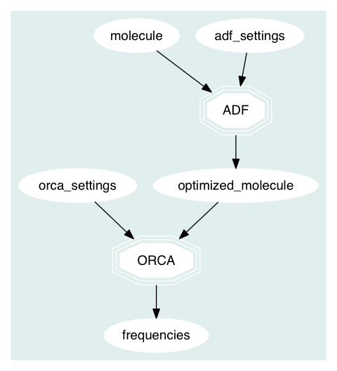
QMflows automatically identify the dependencies between computations and run them in the correct order (if possible in parallel).
Restarting a simulation
If you are running many computationally expensive calculations in a supercomputer, it can happen that the computations take more time than that allowed by the resource manager in your supercomputer and the workflows gets cancel. But do not worry, you do not need to re-run all the computations. Fortunately, QMflows offers a mechanism to restart the workflow computations.
When running a workflow you will see that QMflows creates a set of files called cache. These files contain the information about the workflow and its calculation. In order to restart a workflow you only need to relaunch it, that’s it!
Advanced Examples
Conditional Workflows
from noodles import gather
from qmflows import dftb, adf, orca, run, Settings, templates, molkit, find_first_job

# This examples illustrates the possibility to use different packages interchangeably.
# Analytical frequencies are not available for B3LYP in ADF
# This workflow captures the resulting error and submits the same job to ORCA.

# Define the condition for a successful calculation
def is_successful(result):
    return result.status not in ["failed", "crashed"]

# Generate water molecule
water = molkit.from_smiles('[OH2]', forcefield='mmff')

# Pre-optimize the water molecule
opt_water = dftb(
     templates.geometry, water, job_name="dftb_geometry")

jobs = []

# Generate freq jobs for 3 functionals
for functional in ['pbe', 'b3lyp', 'blyp']:
    s=Settings()
    s.basis = 'DZ'
    s.functional = functional
    # Try to perform the jobs with adf or orca
    # take result from  first successful calculation
    freqjob = find_first_job(
          is_successful, [adf, orca], templates.freq.overlay(s),
          opt_water.molecule, job_name=functional)
    jobs.append(freqjob)

# Run workflow
results = run(gather(*jobs), n_processes=1)
After running the above script you have a table like
pbe     1533.267   3676.165   3817.097
b3lyp   1515.799   3670.390   3825.813
blyp    1529.691   3655.573   3794.110
Non-adiabatic couplings
qmflows-namd is a package based on QMflows to compute the Non-adiabatic couplings for large system involving thr use of QMflows, Cython and Numpy.
Exception Handling
Suppose you have a set of non-dependent calculations, for example single point calculations coming from a molecular dynamic trajectory, as shown in the figure below 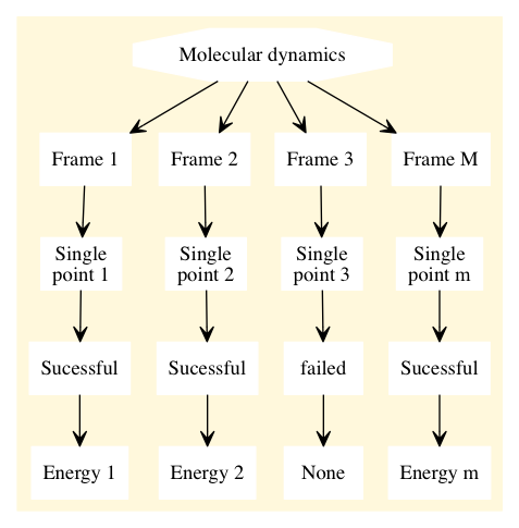
If one of the single point calculations fails, the rest of the point in the workflow will keep on running and the failed job will return a None value for the requested property.
If the single point calculation would be the dependency of another quantum calculation then the computation will crash.